trikit Quickstart Guide
- Release
0.3.3
trikit is a collection of Loss Reserving utilities developed to facilitate Actuarial analysis in Python, with particular emphasis on automating the basic techniques generally used for estimating unpaid claim liabilities. trikit’s core data structure is the triangle, which comes in both incremental and cumulative variants. trikit’s triangle objects inherit directly from Pandas DataFrame, so all of the familiar methods and attributes used when working in Pandas can be be applied to trikit triangle objects.
Along with the core IncrTriangle and CumTriangle data structures,
trikit exposes a number of common methods for estimating unpaid claim liabilities,
as well as techniques to quantify variability around those estimates.
Currently available reserve estimators are BaseChainLadder, MackChainLadder
and BootstrapChainLadder. Refer to the examples below for sample use cases.
Finally, in addition to the library’s core Chain Ladder functionality, trikit
exposes a convenient interface that links to the Casualty Actuarial Society’s
Schedule P Loss Rerserving Database. The database contains information on
losses across a number of lines of business for all property-casualty insurers
that write business in the U.S. More information related to the the Schedule P
Loss Reserving Database can be found here.
Installation
trikit can be installed by running:
$ python -m pip install trikit
Quickstart
We begin by loading the RAA sample dataset, which represents Automatic Factultative business in General Liability provided by the Reinsurance Association of America. Sample datasets are loaded as DataFrame objects, and always represent incremental losses. Sample datasets can be loaded as follows:
In [1]: import trikit
In [2]: raa = trikit.load("raa")
In [3]: raa.head()
Out[3]:
   origin  dev  value
0    1981    1   5012
1    1981    2   3257
2    1981    3   2638
3    1981    4    898
4    1981    5   1734
A list of available datasets can be obtained by calling get_datasets:
In [4]: trikit.get_datasets()
Out[4]: ['amw09', 'autoliab', 'glre', 'raa', 'singinjury', 'singproperty', 'ta83']
Any of the datasets listed above can be read in the same way using
trikit.load. Note that sample datasets can be returned as triangle objects directly. For
example, the RAA dataset can be returned as a cumulative triangle as follows:
In [5]: tri = trikit.load("raa", tri_type="cum")
In [6]: tri
Out[6]:
        1      2      3      4      5      6      7      8      9      10
1981 5,012  8,269 10,907 11,805 13,539 16,181 18,009 18,608 18,662 18,834
1982   106  4,285  5,396 10,666 13,782 15,599 15,496 16,169 16,704    nan
1983 3,410  8,992 13,873 16,141 18,735 22,214 22,863 23,466    nan    nan
1984 5,655 11,555 15,766 21,266 23,425 26,083 27,067    nan    nan    nan
1985 1,092  9,565 15,836 22,169 25,955 26,180    nan    nan    nan    nan
1986 1,513  6,445 11,702 12,935 15,852    nan    nan    nan    nan    nan
1987   557  4,020 10,946 12,314    nan    nan    nan    nan    nan    nan
1988 1,351  6,947 13,112    nan    nan    nan    nan    nan    nan    nan
1989 3,133  5,395    nan    nan    nan    nan    nan    nan    nan    nan
1990 2,063    nan    nan    nan    nan    nan    nan    nan    nan    nan
Working with Triangles
Triangles are created by calling the totri function. Available arguments
are:
data: The dataset to transform into a triangle instance.tri_type: {“cum”, “incr”} Specifies the type of triangle to create.data_format: {“cum”, “incr”} Specifies how losses are represented with the input datasetdata.data_shape: {“tabular”, “triangle”} Specifies whether input datasetdatarepresents tabular loss data with columns “origin”, “dev” and “value”, or data already structured as a loss triangle with columns corresponding to development periods.origin: The column name indatacorresponding to accident year. Ignored ifdata_shape="triangle".dev: The column name indatacorresponding to development period. Ignored ifdata_shape="triangle".value: The column name indatacorresponding to the measure of interest. Ignored ifdata_shape="triangle".
Next we demonstrate how to create triangles using totri and various
combinations of the arguments listed above.
Example 1: Create a cumulative loss triangle from tabular incremental data
Referring again to the RAA dataset, let’s create a cumulative loss triangle.
We mentioned above that trikit sample datasets are Pandas DataFrames which
reflect incremental losses, so data_format="incr" and data_shape="tabular",
both of which are defaults. Also, the default for tri_type is "cum", so the
only argument required to pass into totri is the input dataset data:
In [1]: import pandas as pd
In [2]: from trikit import load, totri
In [3]: raa = load("raa")
In [4]: tri = totri(raa)
In [5]: tri
Out[5]:
        1      2      3      4      5      6      7      8      9      10
1981 5,012  8,269 10,907 11,805 13,539 16,181 18,009 18,608 18,662 18,834
1982   106  4,285  5,396 10,666 13,782 15,599 15,496 16,169 16,704    nan
1983 3,410  8,992 13,873 16,141 18,735 22,214 22,863 23,466    nan    nan
1984 5,655 11,555 15,766 21,266 23,425 26,083 27,067    nan    nan    nan
1985 1,092  9,565 15,836 22,169 25,955 26,180    nan    nan    nan    nan
1986 1,513  6,445 11,702 12,935 15,852    nan    nan    nan    nan    nan
1987   557  4,020 10,946 12,314    nan    nan    nan    nan    nan    nan
1988 1,351  6,947 13,112    nan    nan    nan    nan    nan    nan    nan
1989 3,133  5,395    nan    nan    nan    nan    nan    nan    nan    nan
1990 2,063    nan    nan    nan    nan    nan    nan    nan    nan    nan
tri is an instance of trikit.triangle.CumTriangle, which inherits from pandas.DataFrame:
In [6]: type(tri)
Out[6]: trikit.triangle.CumTriangle
In [7]: isinstance(tri, pd.DataFrame)
Out[7]: True
This means that all of the functionality exposed by DataFrame objects gets inherited
by triangle objects. For example, to access the first column of tri:
In [8]: tri.loc[:,1]
Out[8]:
1981   5012.00000
1982    106.00000
1983   3410.00000
1984   5655.00000
1985   1092.00000
1986   1513.00000
1987    557.00000
1988   1351.00000
1989   3133.00000
1990   2063.00000
Name: 1, dtype: float64
Triangle objects offer a number of methods useful in Actuarial reserving
contexts. To extract the latest diagonal, call tri.latest:
In [9]: tri.latest
Out[9]:
   origin  dev      latest
0    1981   10 18834.00000
1    1982    9 16704.00000
2    1983    8 23466.00000
3    1984    7 27067.00000
4    1985    6 26180.00000
5    1986    5 15852.00000
6    1987    4 12314.00000
7    1988    3 13112.00000
8    1989    2  5395.00000
9    1990    1  2063.00000
Calling tri.a2a produces a DataFrame of age-to-age factors:
In[10]: tri.a2a
Out[10]:
            1       2       3       4       5       6       7       8       9
1981  1.64984 1.31902 1.08233 1.14689 1.19514 1.11297 1.03326 1.00290 1.00922
1982 40.42453 1.25928 1.97665 1.29214 1.13184 0.99340 1.04343 1.03309     nan
1983  2.63695 1.54282 1.16348 1.16071 1.18570 1.02922 1.02637     nan     nan
1984  2.04332 1.36443 1.34885 1.10152 1.11347 1.03773     nan     nan     nan
1985  8.75916 1.65562 1.39991 1.17078 1.00867     nan     nan     nan     nan
1986  4.25975 1.81567 1.10537 1.22551     nan     nan     nan     nan     nan
1987  7.21724 2.72289 1.12498     nan     nan     nan     nan     nan     nan
1988  5.14212 1.88743     nan     nan     nan     nan     nan     nan     nan
1989  1.72199     nan     nan     nan     nan     nan     nan     nan     nan
Calling tri.a2a_avgs produces a table of candidate loss development factors,
which contains arithmetic, geometric and weighted age-to-age averages for a
number of different periods:
In[11]: tri.a2a_avgs()
Out[11]:
                    1       2       3       4       5       6       7       8       9
simple-1      1.72199 1.88743 1.12498 1.22551 1.00867 1.03773 1.02637 1.03309 1.00922
simple-2      3.43205 2.30516 1.11517 1.19815 1.06107 1.03347 1.03490 1.01799 1.00922
simple-3      4.69378 2.14200 1.21009 1.16594 1.10261 1.02011 1.03436 1.01799 1.00922
simple-4      4.58527 2.02040 1.24478 1.16463 1.10992 1.04333 1.03436 1.01799 1.00922
simple-5      5.42005 1.88921 1.22852 1.19013 1.12696 1.04333 1.03436 1.01799 1.00922
simple-6      4.85726 1.83148 1.35321 1.18293 1.12696 1.04333 1.03436 1.01799 1.00922
simple-7      4.54007 1.74973 1.31451 1.18293 1.12696 1.04333 1.03436 1.01799 1.00922
simple-8      9.02563 1.69589 1.31451 1.18293 1.12696 1.04333 1.03436 1.01799 1.00922
all-simple    8.20610 1.69589 1.31451 1.18293 1.12696 1.04333 1.03436 1.01799 1.00922
geometric-1   1.72199 1.88743 1.12498 1.22551 1.00867 1.03773 1.02637 1.03309 1.00922
geometric-2   2.97568 2.26699 1.11513 1.19783 1.05977 1.03346 1.03487 1.01788 1.00922
geometric-3   3.99805 2.10529 1.20296 1.16483 1.10019 1.01993 1.03433 1.01788 1.00922
geometric-4   4.06193 1.98255 1.23788 1.16380 1.10802 1.04244 1.03433 1.01788 1.00922
geometric-5   4.73672 1.83980 1.22263 1.18840 1.12492 1.04244 1.03433 1.01788 1.00922
geometric-6   4.11738 1.78660 1.32455 1.18138 1.12492 1.04244 1.03433 1.01788 1.00922
geometric-7   3.86345 1.69952 1.28688 1.18138 1.12492 1.04244 1.03433 1.01788 1.00922
geometric-8   5.18125 1.64652 1.28688 1.18138 1.12492 1.04244 1.03433 1.01788 1.00922
all-geometric 4.56261 1.64652 1.28688 1.18138 1.12492 1.04244 1.03433 1.01788 1.00922
weighted-1    1.72199 1.88743 1.12498 1.22551 1.00867 1.03773 1.02637 1.03309 1.00922
weighted-2    2.75245 2.19367 1.11484 1.19095 1.05838 1.03381 1.03326 1.01694 1.00922
weighted-3    3.24578 2.05376 1.23215 1.15721 1.09340 1.02395 1.03326 1.01694 1.00922
weighted-4    3.47986 1.91259 1.26606 1.15799 1.09987 1.04193 1.03326 1.01694 1.00922
weighted-5    4.23385 1.74821 1.24517 1.17519 1.11338 1.04193 1.03326 1.01694 1.00922
weighted-6    3.30253 1.70935 1.29886 1.17167 1.11338 1.04193 1.03326 1.01694 1.00922
weighted-7    3.16672 1.67212 1.27089 1.17167 1.11338 1.04193 1.03326 1.01694 1.00922
weighted-8    3.40156 1.62352 1.27089 1.17167 1.11338 1.04193 1.03326 1.01694 1.00922
all-weighted  2.99936 1.62352 1.27089 1.17167 1.11338 1.04193 1.03326 1.01694 1.00922
We can obtain a reference to an incremental representation of the cumulative triangle
by calling tri.to_incr:
In[12]: tri.to_incr()
Out[12]:
        1     2     3     4     5     6     7   8   9   10
1981 5,012 3,257 2,638   898 1,734 2,642 1,828 599  54 172
1982   106 4,179 1,111 5,270 3,116 1,817  -103 673 535 nan
1983 3,410 5,582 4,881 2,268 2,594 3,479   649 603 nan nan
1984 5,655 5,900 4,211 5,500 2,159 2,658   984 nan nan nan
1985 1,092 8,473 6,271 6,333 3,786   225   nan nan nan nan
1986 1,513 4,932 5,257 1,233 2,917   nan   nan nan nan nan
1987   557 3,463 6,926 1,368   nan   nan   nan nan nan nan
1988 1,351 5,596 6,165   nan   nan   nan   nan nan nan nan
1989 3,133 2,262   nan   nan   nan   nan   nan nan nan nan
1990 2,063   nan   nan   nan   nan   nan   nan nan nan nan
Example 2: Create an incremental loss triangle from tabular incremental data
The call to totri is identical to Example #1, but we change tri_type from
“cum” to “incr”:
In [1]: import pandas as pd
In [2]: from trikit import load, totri
In [3]: raa = load("raa")
In [4]: tri = totri(raa, tri_type="incr")
In [5]: type(tri)
Out[5]: trikit.triangle.IncrTriangle
In [6]: tri
Out[6]:
        1     2     3     4     5     6     7   8   9   10
1981 5,012 3,257 2,638   898 1,734 2,642 1,828 599  54 172
1982   106 4,179 1,111 5,270 3,116 1,817  -103 673 535 nan
1983 3,410 5,582 4,881 2,268 2,594 3,479   649 603 nan nan
1984 5,655 5,900 4,211 5,500 2,159 2,658   984 nan nan nan
1985 1,092 8,473 6,271 6,333 3,786   225   nan nan nan nan
1986 1,513 4,932 5,257 1,233 2,917   nan   nan nan nan nan
1987   557 3,463 6,926 1,368   nan   nan   nan nan nan nan
1988 1,351 5,596 6,165   nan   nan   nan   nan nan nan nan
1989 3,133 2,262   nan   nan   nan   nan   nan nan nan nan
1990 2,063   nan   nan   nan   nan   nan   nan nan nan nan
tri now represents RAA losses in incremental format.
It is possible to obtain a cumulative representation of an incremental triangle
object by calling tri.to_cum:
In [7]: tri.to_cum()
Out[7]:
        1      2      3      4      5      6      7      8      9      10
1981 5,012  8,269 10,907 11,805 13,539 16,181 18,009 18,608 18,662 18,834
1982   106  4,285  5,396 10,666 13,782 15,599 15,496 16,169 16,704    nan
1983 3,410  8,992 13,873 16,141 18,735 22,214 22,863 23,466    nan    nan
1984 5,655 11,555 15,766 21,266 23,425 26,083 27,067    nan    nan    nan
1985 1,092  9,565 15,836 22,169 25,955 26,180    nan    nan    nan    nan
1986 1,513  6,445 11,702 12,935 15,852    nan    nan    nan    nan    nan
1987   557  4,020 10,946 12,314    nan    nan    nan    nan    nan    nan
1988 1,351  6,947 13,112    nan    nan    nan    nan    nan    nan    nan
1989 3,133  5,395    nan    nan    nan    nan    nan    nan    nan    nan
1990 2,063    nan    nan    nan    nan    nan    nan    nan    nan    nan
Example 3: Create a cumulative loss triangle from data formatted as a triangle
There may be situations in which data is already formatted as a triangle,
and we’re interested in creating a triangle instance from this data.
In the next example, we create a DataFrame with the same shape as a triangle,
which we then pass into totri with data_shape="triangle" to obtain a
cumulative triangle instance:
In [1]: import pandas as pd
In [2]: from trikit import load, totri
In [3]: dftri = pd.DataFrame({
            1:[1010, 1207, 1555, 1313, 1905],
            2:[767, 1100, 1203, 900, np.NaN],
            3:[444, 623, 841, np.NaN, np.NaN],
            4:[239, 556, np.NaN, np.NaN, np.NaN],
            5:[80, np.NaN, np.NaN, np.NaN, np.NaN],
            }, index=list(range(1, 6))
            )
In [4]: dftri
Out[4]:
      1     2    3    4   5
1  1010.  767. 444. 239. 80.
2  1207. 1100. 623. 556. nan
3  1555. 1203. 841. nan  nan
4  1313.  900. nan  nan  nan
5  1905.  nan  nan  nan  nan

In [5]: tri = totri(dftri, data_shape="triangle")
In [6]: type(tri)
Out[6]: trikit.triangle.CumTriangle
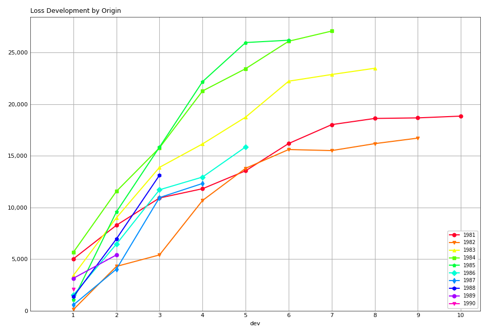
trikit cumulative triangle instances expose a plot method, which generates a faceted plot by origin representing the progression of cumulative losses to date by development period. The exhibit can be obtained as follows:
In [5]: tri.plot()
Which yields:
Reserve Estimators
trikit includes a number of reserve estimators. Let’s refer to the CAS Loss Reserving
Dastabase (lrdb) included with trikit, focusing on grcode=1767 and lob="comauto"
(grcode uniquely identifies each company in the database. To obtain a full list of
grcodes and associated companies, use trikit.get_lrdb_specs; to obtain a list
of availavble lines of business (lobs), use trikit.get_lrdb_lobs):
In [1]: from trikit import load_lrdb, totri
In [2]: df = load_lrdb(lob="comauto", grcode=1767)
In [3]: tri = totri(df)
In [4]: tri
          1       2       3       4       5         6         7         8         9         10
1988 110,231 263,079 431,216 611,278 797,428   985,570 1,174,922 1,366,229 1,558,096 1,752,096
1989 121,678 279,896 456,640 644,767 837,733 1,033,837 1,233,015 1,432,670 1,633,619       nan
1990 123,376 298,615 500,570 714,683 934,671 1,157,979 1,383,820 1,610,193       nan       nan
1991 117,457 280,058 463,396 662,003 865,401 1,071,271 1,278,228       nan       nan       nan
1992 124,611 291,399 481,170 682,203 889,029 1,101,390       nan       nan       nan       nan
1993 137,902 323,854 533,211 753,639 980,180       nan       nan       nan       nan       nan
1994 150,582 345,110 561,315 792,392     nan       nan       nan       nan       nan       nan
1995 150,511 345,241 560,278     nan     nan       nan       nan       nan       nan       nan
1996 142,301 326,584     nan     nan     nan       nan       nan       nan       nan       nan
1997 143,970     nan     nan     nan     nan       nan       nan       nan       nan       nan
Similar to load, load_lrdb also accepts a tri_type argument, which returns the lrdb subset
as an incremental or cumulative triangle:
In [5]: tri = load_lrdb(tri_type="cum", lob="comauto", grcode=1767)
To obtain base chain ladder reserve estimates, call the cumulative triangle’s
base_cl method:
In [5]: result = tri.base_cl()
In [6]: result
Out[6]:
      maturity     cldf emergence     latest   ultimate    reserve
1988        10  1.00000   1.00000  1,752,096  1,752,096          0
1989         9  1.12451   0.88928  1,633,619  1,837,022    203,403
1990         8  1.28233   0.77983  1,610,193  2,064,802    454,609
1991         7  1.49111   0.67064  1,278,228  1,905,977    627,749
1992         6  1.77936   0.56200  1,101,390  1,959,771    858,381
1993         5  2.20146   0.45425    980,180  2,157,822  1,177,642
1994         4  2.87017   0.34841    792,392  2,274,299  1,481,907
1995         3  4.07052   0.24567    560,278  2,280,624  1,720,346
1996         2  6.68757   0.14953    326,584  2,184,053  1,857,469
1997         1 15.62506   0.06400    143,970  2,249,541  2,105,571
total               nan       nan 10,178,930 20,666,007 10,487,077
The result is of type BaseChainLadderResult. The columns
of the result can be obtained in total or individually. The result above
can be returned as a DataFrame by calling result.summary:
In [7]: result.summary
Out[7]:
      maturity       cldf  emergence      latest      ultimate       reserve
1988        10   1.000000   1.000000   1752096.0  1.752096e+06  0.000000e+00
1989         9   1.124511   0.889275   1633619.0  1.837022e+06  2.034034e+05
1990         8   1.282332   0.779829   1610193.0  2.064802e+06  4.546094e+05
1991         7   1.491108   0.670642   1278228.0  1.905977e+06  6.277486e+05
1992         6   1.779362   0.561999   1101390.0  1.959771e+06  8.583811e+05
1993         5   2.201455   0.454245    980180.0  2.157822e+06  1.177642e+06
1994         4   2.870169   0.348412    792392.0  2.274299e+06  1.481907e+06
1995         3   4.070523   0.245669    560278.0  2.280624e+06  1.720346e+06
1996         2   6.687568   0.149531    326584.0  2.184053e+06  1.857469e+06
1997         1  15.625064   0.064000    143970.0  2.249541e+06  2.105571e+06
total                 NaN        NaN  10178930.0  2.066601e+07  1.048708e+07
To access the reserve estimates as a Series, call result.reserve:
In [8]: result.reserve
Out[8]:
1988            0.0
1989       203403.0
1990       454609.0
1991       627749.0
1992       858381.0
1993      1177642.0
1994      1481907.0
1995      1720346.0
1996      1857469.0
1997      2105571.0
total    10487077.0
Name: reserve, dtype: float64
base_cl accepts two optional arguments:
tail: The tail factor, which defaults to 1.0.sel: Loss development factors, which defaults to “all-weighted”.selcan be either a string corresponding to a pre-computed pattern available intri.a2a_avgs().index, or a custom set of loss development factors as a numpy array or Pandas Series.
Example #2 demonstrated how to access a number of candidate loss development patterns
by calling tri.a2a_avgs. Available pre-computed options for sel can be any
value present in tri.a2a_avgs’s index. To obtain a list of available pre-computed
loss development factors by name, run:
In [9]: tri.a2a_avgs().index.tolist()
Out[9]:
['simple-1', 'simple-2', 'simple-3', 'simple-4', 'simple-5', 'simple-6', 'simple-7',
'simple-8', 'all-simple', 'geometric-1', 'geometric-2', 'geometric-3', 'geometric-4',
'geometric-5', 'geometric-6', 'geometric-7', 'geometric-8', 'all-geometric',
'weighted-1', 'weighted-2', 'weighted-3', 'weighted-4', 'weighted-5', 'weighted-6',
'weighted-7', 'weighted-8', 'all-weighted']
If instead of all-weighted, a 5-year geometric loss development pattern is
preferred, along with a tail factor of 1.015, the call to base_cl would be modified
as follows:
In[10]: tri.base_cl(sel="geometric-5", tail=1.015)
Out[10]:
      maturity     cldf emergence     latest   ultimate    reserve
1988        10  1.01500   0.98522  1,752,096  1,778,377     26,281
1989         9  1.14138   0.87613  1,633,619  1,864,578    230,959
1990         8  1.30157   0.76830  1,610,193  2,095,778    485,585
1991         7  1.51344   0.66075  1,278,228  1,934,517    656,289
1992         6  1.80591   0.55374  1,101,390  1,989,009    887,619
1993         5  2.23416   0.44760    980,180  2,189,878  1,209,698
1994         4  2.91249   0.34335    792,392  2,307,832  1,515,440
1995         3  4.13521   0.24183    560,278  2,316,869  1,756,591
1996         2  6.78292   0.14743    326,584  2,215,194  1,888,610
1997         1 15.69149   0.06373    143,970  2,259,103  2,115,133
total               nan       nan 10,178,930 20,951,135 10,772,205
If sel is a Series or numpy ndarray, a check will first be made to ensure the LDFs
have the requiste number of elements. The provided LDFs should not include a tail factor.
Next, reserves are estimated with the chain ladder along with an external set of LDFs
using the same loss reserve database subset (grcode=1767 and lob="commauto"):
In[11]: tri = load_lrdb(tri_type="cum", lob="commauto", grcode=1767)
In[12]: ldfs = np.asarray([2.75, 1.55, 1.50, 1.25, 1.15, 1.075, 1.03, 1.02, 1.01])
In[13]: cl = tri.base_cl(sel=ldfs)
In[14]: cl
Out[14]:
      maturity     cldf emergence     latest   ultimate   reserve
1988        10  1.00000   1.00000  1,752,096  1,752,096         0
1989         9  1.01000   0.99010  1,633,619  1,649,955    16,336
1990         8  1.03020   0.97069  1,610,193  1,658,821    48,628
1991         7  1.06111   0.94241  1,278,228  1,356,335    78,107
1992         6  1.14069   0.87666  1,101,390  1,256,343   154,953
1993         5  1.31179   0.76232    980,180  1,285,793   305,613
1994         4  1.63974   0.60985    792,392  1,299,317   506,925
1995         3  2.45961   0.40657    560,278  1,378,066   817,788
1996         2  3.81240   0.26230    326,584  1,245,068   918,484
1997         1 10.48409   0.09538    143,970  1,509,394 1,365,424
total               nan       nan 10,178,930 14,391,188 4,212,258
If ldfs is not of the correct length (length n-1 for a triangle
having n development periods), ValueError is raised:
In[15]: ldfs = np.asarray([2.75, 1.55, 1.50, 1.25, 1.15, 1.075, 1.03])
In[16]: result = tri._base_cl(sel=ldfs)
Traceback (most recent call last):
File "trikit\chainladder\base.py", line 117, in __call__
ValueError: sel has 7 values, LDF overrides require 9.
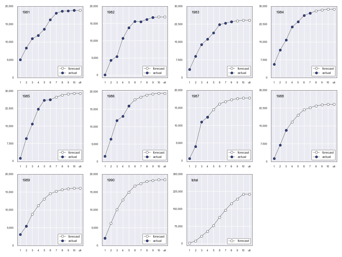
A faceted plot by origin combining actuals and forcasts can be obtained by calling
result’s plot method:
In [17]: result = tri.base_cl(sel="geometric-5", tail=1.015)
In [18]: result.plot()
Which produces the following:
Quantifying Reserve Variability
The Base Chain Ladder method provides an estimate by origin and in total of future outstanding claim liabilities, but offers no indication of the variability around those point estimates. We can obtain quantiles of the predictive distribution of reserve estimates through a number of trikit estimators.
Mack Chain Ladder
The Mack Chain Ladder is a distribution free model which estimates the first
two moments of standard chain ladder forecasts. Within trikit, the Mack Chain
Ladder is encapsulated within a cumulative triangle’s mack_cl method.
mack_cl accepts a number of optional arguments:
alpha: Controls how loss development factors are computed. Can be 0, 1 or 2. Whenalpha=0, LDFs are computed as the straight average of observed individual link ratios. Whenalpha=1, the historical Chain Ladder age-to-age factors are computed. Whenalpha=2, a regression of :math: C_{k+1} on :math: C_{k} with 0 intercept is performed. Default is 1.dist: Either “norm” or “lognorm”. Represents the selected distribution to approximate the true distribution of reserves by origin period and in aggregate. Settingdist="norm"specifies a normal distribution.dist="lognorm"assumes a log-normal distribution. Default is “lognorm”.q: Quantile or sequence of quantiles to compute, which must be between 0 and 1 inclusive. Default is [.75, .95].two_sided: Whether the two_sided interval should be included in summary output. For example, iftwo_sided==Trueandq=.95, then the 2.5th and 97.5th quantiles of the estimated reserve distribution will be returned ((1 - .95) / 2, (1 + .95) / 2). When False, only the specified quantile(s) will be computed. Default value is False.
Using the ta83 sample dataset, calling mack_cl with default arguments yields:
In [1]: from trikit import load, totri
In [2]: tri = load("ta83", tri_type="cum")
In [3]: mcl = tri.mack_cl()
In [4]: mcl
Out[4]:
      maturity     cldf emergence     latest   ultimate    reserve std_error      cv        75%        95%
1           10  1.00000   1.00000  3,901,463  3,901,463          0         0     nan        nan        nan
2            9  1.01772   0.98258  5,339,085  5,433,719     94,634    75,535 0.79818    118,760    234,717
3            8  1.09564   0.91271  4,909,315  5,378,826    469,511   121,700 0.25921    539,788    691,334
4            7  1.15466   0.86605  4,588,268  5,297,906    709,638   133,551 0.18820    790,911    947,870
5            6  1.25428   0.79727  3,873,311  4,858,200    984,889   261,412 0.26542  1,135,100  1,462,149
6            5  1.38450   0.72228  3,691,712  5,111,171  1,419,459   411,028 0.28957  1,651,045  2,174,408
7            4  1.62520   0.61531  3,483,130  5,660,771  2,177,641   558,356 0.25640  2,500,779  3,194,587
8            3  2.36858   0.42219  2,864,498  6,784,799  3,920,301   875,430 0.22331  4,439,877  5,499,652
9            2  4.13870   0.24162  1,363,294  5,642,266  4,278,972   971,385 0.22701  4,853,918  6,033,399
10           1 14.44662   0.06922    344,014  4,969,838  4,625,824 1,363,376 0.29473  5,390,689  7,133,025
total               nan       nan 34,358,090 53,038,959 18,680,869 2,447,318 0.13101 20,226,192 22,955,604
Quantiles of the estimated reserve distribution can be obtained by calling get_quantiles.
q can be either a single float or an array of floats representing the percentiles of
interest (which must fall within [0, 1]):
In [5]: mcl.get_quantiles(q=[.05, .10, .25, .50, .75, .90, .95])
Out[5]:
             5th       10th       25th       50th       75th       90th       95th
1            nan        nan        nan        nan        nan        nan        nan
2        23306.0    30078.0    46063.0    73962.0   118760.0   181873.0   234717.0
3       298788.0   327792.0   382673.0   454491.0   539788.0   630163.0   691334.0
4       513108.0   549091.0   614936.0   697395.0   790911.0   885754.0   947870.0
5       619750.0   681372.0   798314.0   951928.0  1135100.0  1329915.0  1462149.0
6       854941.0   947780.0  1125948.0  1363448.0  1651045.0  1961416.0  2174408.0
7      1392853.0  1526576.0  1779281.0  2109405.0  2500779.0  2914751.0  3194587.0
8      2661766.0  2883868.0  3297115.0  3826066.0  4439877.0  5076093.0  5499652.0
9      2885978.0  3130850.0  3587259.0  4172800.0  4853918.0  5561511.0  6033399.0
10     2760122.0  3065251.0  3652226.0  4437118.0  5390689.0  6422971.0  7133025.0
total 14945656.0 15671023.0 16962489.0 18522596.0 20226192.0 21893054.0 22955604.0
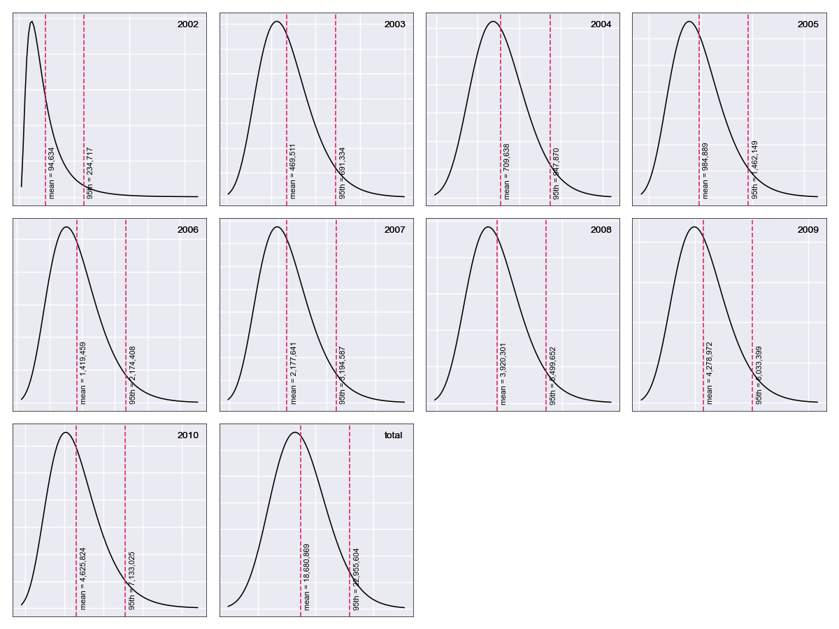
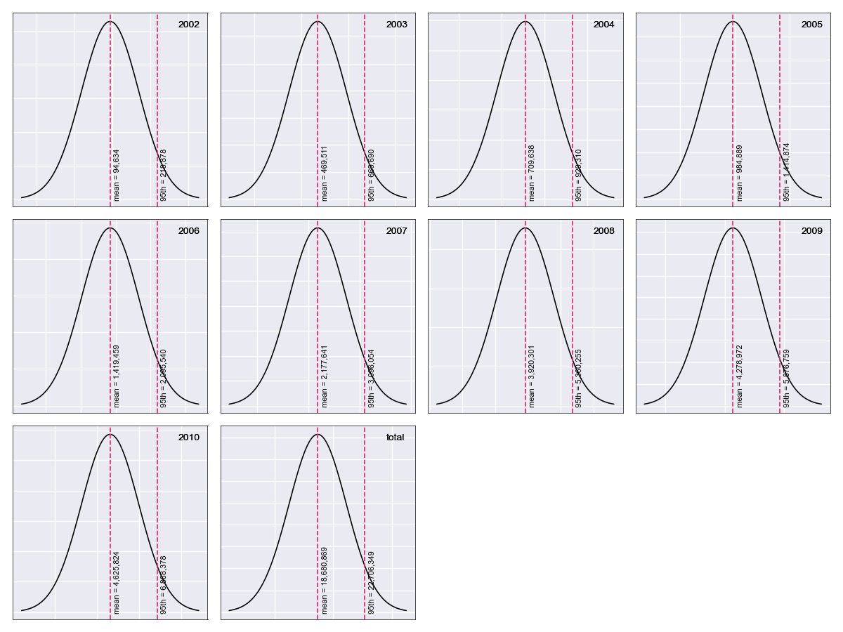
The MackChainLadderResult’s plot method returns a faceted plot of estimated
reserve distributions by origin and in total. The mean is highlighted, along with
any quantiles passed to the plot method via q. We can compare the estimated distributions
when dist="lognorm" vs. dist="norm", highlighting the mean and 95th percentile.
First we take a look at dist="lognorm":
In [7]: mcl.plot()
Which produces the following:
Next we produce the same exhibit, this time setting dist="norm":
In [8]: mcl = tri.mack_cl(dist="norm")
In [9]: mcl.plot()
Which generates:
Testing for Development Period Correlation
In 2 Appendix G., Mack proposes an approximate test to assess whether one
of the basic Chain Ladder assumptions holds, namely that subsequent development
periods are uncorrelated. The test can be performed via MackChainLadderResult`’s
devp_corr_test method. We next apply the test to the RAA dataset:
In [1]: from trikit import load, totri
In [2]: tri = load("raa", tri_type="cum")
In [3]: mcl = tri.mack_cl()
In [4]: mcl.devp_corr_test()
Out[4]: ((-0.12746658149149367, 0.12746658149149367), 0.0695578231292517)
devp_corr_test returns a 2-tuple: The first element represents the bounds
of the test interval ((-0.127, 0.127)). The second element is the test statistic
for the triangle under consideration. In this example, the test statistic falls
within the bounds of the test interval, therefore we do not reject the null-hypothesis
of having uncorrelated development factors. If the test statistic falls outside the
interval, the correlations should be analyzed in more detail. Refer to 2 for more
information.
Testing for Calendar Year Effects
In 2 Appendix H., Mack proposes a test to assess the independence of the origin
periods. This test can be performed via MackChainLadderResult’s cy_effects_test
method. Again using the RAA dataset:
In [1]: from trikit import load, totri
In [2]: tri = load("raa", tri_type="cum")
In [3]: mcl = tri.mack_cl()
In [4]: mcl.cy_effects_test()
Out[4]: ((8.965613354894957, 16.78438664510504), 14.0)
Similar to devp_corr_test, cy_effects_test returns a 2-tuple, with the first
element representing the bounds of the test interval ((8.97, 16.78)) and the second
element the test statistic. In this example, the test statistic falls within the
bounds of thew test interval, therefore we do not reject the null-hypothesis of not
having significant calendar year influences. Refer to 2 for more
information.
Mack Chain Ladder Diagnostics
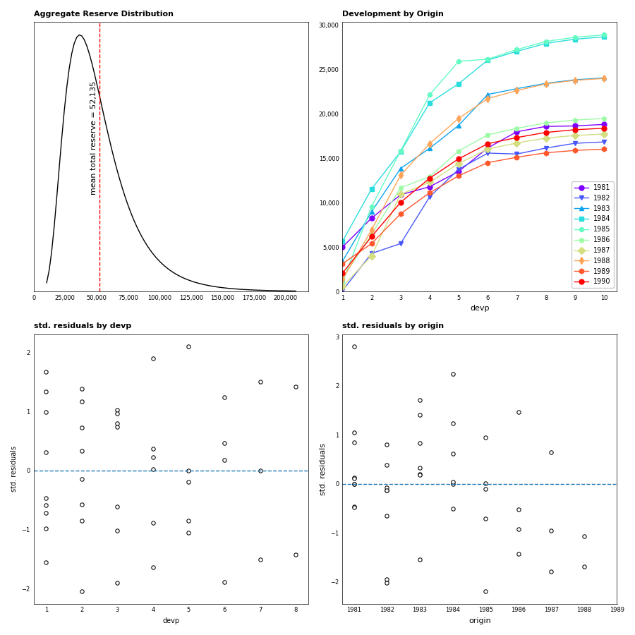
MackChainLadderResult exposes a diagnostics method, which generates a faceted plot
that includes the estimated aggregate reserve distribution, development by origin
and standardized residuals by development period and by origin:
In [1]: from trikit import load, totri
In [2]: tri = load("raa", tri_type="cum")
In [3]: mcl = tri.mack_cl()
In [4]: mcl.diagnostics()
Which produces the following:
Bootstrap Chain Ladder
The purpose of the Bootstrap Chain Ladder is to estimate the predicition error of
the total reserve estimate and to approximate the predictive distribution.
Within trikit, the Bootstrap Chain Ladder is encapsulated within a cumulative
triangle’s boot_cl method. boot_cl accepts a number of optional arguments:
sims: The number of bootstrap iterations to perform. Default value is 1000.q: Quantile or sequence of quantiles to compute, which must be between 0 and 1 inclusive. Default value is [.75, .95].procdist: The distribution used to incorporate process variance. Currently, this can only be set to “gamma”. This may change in a future release.two_sided: Whether the two_sided prediction interval should be included in summary output. For example, iftwo_sided=Trueandq=.95, then the 2.5th and 97.5th quantiles of the predictive reserve distribution will be returned [(1 - .95) / 2, (1 + .95) / 2]. When False, only the specified quantile(s) will be included in summary output. Default value is False.parametric: If True, fit standardized residuals to a normal distribution via maximum likelihood, and sample from the parameterized distribution. Otherwise, sample with replacement from the collection of standardized fitted triangle residuals. Default value is False.interpolation: One of {“linear”, “lower”, “higher”, “midpoint”, “nearest”}. Default value is “linear”. Refer to numpy.quantile for more information.random_state: If int, random_state is the seed used by the random number generator; IfRandomStateinstance, random_state is the random number generator; If None, the random number generator is theRandomStateinstance used by np.random. Default value is None.
We next demonstrate the application of the Bootstrap Chain Ladder to the RAA dataset.
The example sets sims=1000, two_sided=False and random_state=516 for reproducibility:
In [1]: from trikit import load, totri
In [2]: df = load("raa", tri_type="cum")
In [3]: bcl = tri.boot_cl(sims=1000, two_sided=False, random_state=516)
In [4]: bcl
Out[4]:
      maturity    cldf emergence  latest ultimate reserve std_error    cv    75%    95%
1981        10 1.00000   1.00000  18,834   18,834       0         0   nan      0      0
1982         9 1.00922   0.99087  16,704   16,863     159       529 3.331    245  1,108
1983         8 1.02631   0.97437  23,466   24,395     929     1,026 1.104  1,101  2,609
1984         7 1.06045   0.94300  27,067   28,648   1,581     1,592 1.007  2,472  4,704
1985         6 1.10492   0.90505  26,180   29,087   2,907     1,883 0.648  3,914  6,341
1986         5 1.23020   0.81288  15,852   19,762   3,910     1,931 0.494  4,892  7,114
1987         4 1.44139   0.69377  12,314   17,738   5,424     2,538 0.468  6,947 10,061
1988         3 1.83185   0.54590  13,112   24,365  11,253     3,980 0.354 13,565 18,735
1989         2 2.97405   0.33624   5,395   16,325  10,930     4,940 0.452 13,870 19,879
1990         1 8.92023   0.11210   2,063   18,973  16,910    11,028 0.652 22,863 37,008
total              nan       nan 160,987  214,989  54,002    14,832 0.275 62,597 80,200
reserve represents the mean of the predicitive distribution of reserve estimates
by origin and in total; 75% and 95% represent quantiles of the estimated distribution.
Additional quantiles of the bootstrapped reserve distribution can be obtained by calling
get_quantiles. q can be either a single float or an array of floats representing the
quantiles of interest (which must fall within [0, 1]). We set lb=0 to set negative quantiles
to 0:
In [5]: bcl.get_quantiles(q=[.05, .10, .25, .75, .90, .95], lb=0)
Out[5]:
          5th    10th    25th    75th    90th    95th
1981      0.0     0.0     0.0     0.0     0.0     0.0
1982      0.0     0.0     0.0   245.0   694.0  1108.0
1983      0.0     0.0    30.0  1101.0  2001.0  2609.0
1984      0.0   142.0   618.0  2472.0  3758.0  4704.0
1985    349.0   693.0  1449.0  3914.0  5234.0  6341.0
1986   1117.0  1454.0  2319.0  4892.0  6348.0  7114.0
1987   1838.0  2396.0  3555.0  6947.0  8832.0 10061.0
1988   5469.0  6452.0  8256.0 13565.0 16339.0 18735.0
1989   3671.0  4892.0  7257.0 13870.0 17667.0 19879.0
1990   1793.0  4278.0  8790.0 22863.0 30904.0 37008.0
total 31588.0 36193.0 43009.0 62597.0 73218.0 80200.0
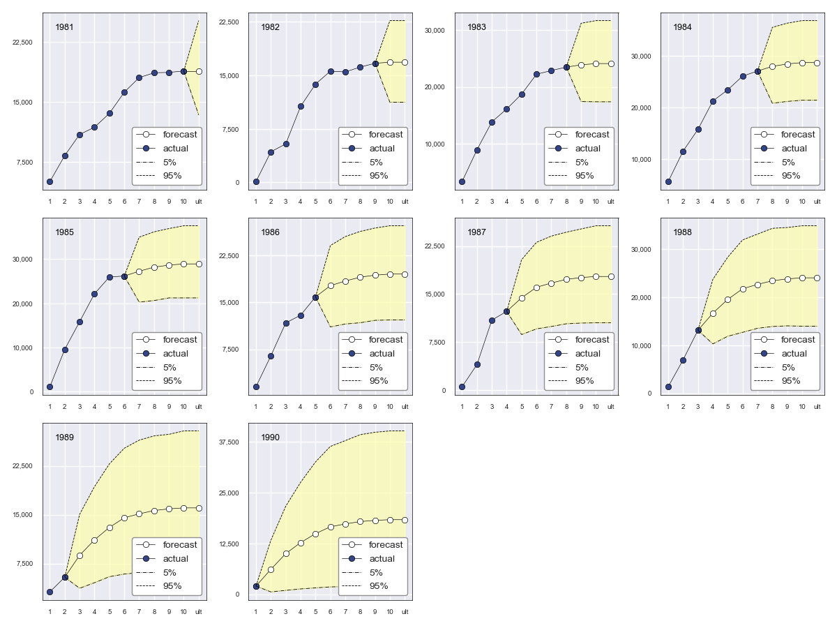
The BoostrapChainLadderResult object exposes two exhibits: The first
is similar to BaseChainLadderResult’s plot, but includes the upper and lower
bounds of the specified percentile of the predictive distribution. To obtain the faceted
plot showing the 5th and 95th quantiles, run:
In [2]: bcl = tri.boot_cl(sims=2500, two_sided=True, random_state=516)
In [2]: bcl.plot(q=.90)
Resulting in:
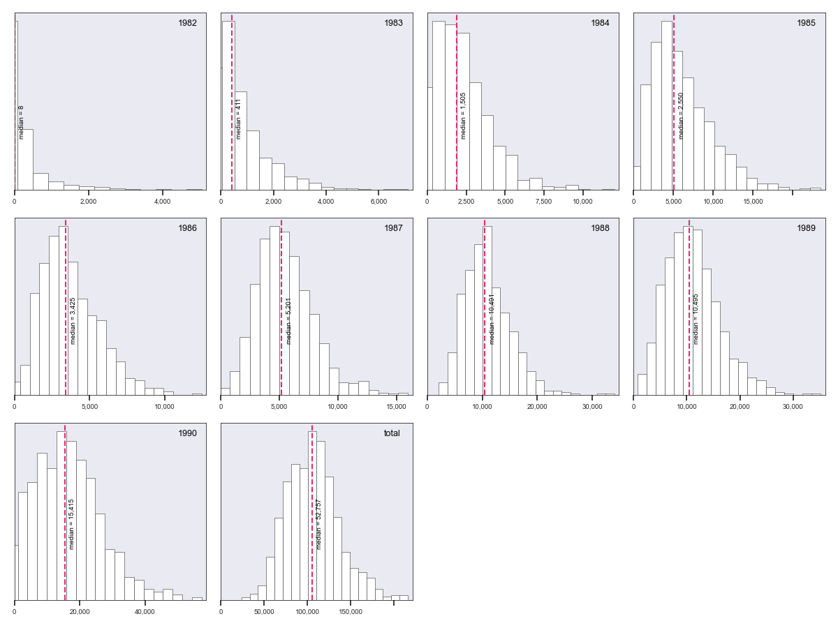
In addition, we can obtain a faceted plot of the distribution of bootstrap samples
by origin and in aggregate by calling BoostrapChainLadderResult’s hist
method:
In [4]: bcl.hist()
Which generates:
There are a number of parameters which control the style of the generated exhibits. Refer to the docstring for more information.
Contact
Please contact james.triveri@gmail.com with suggestions or feature requests.
Footnotes
- 1
https://www.casact.org/research/index.cfm?fa=loss_reserves_data
- 2(1,2,3,4)
Mack, Thomas (1993) Measuring the Variability of Chain Ladder Reserve Estimates, 1993 CAS Prize Paper Competition on ‘Variability of Loss Reserves’.
- 3
Mack, Thomas, (1993), Distribution-Free Calculation of the Standard Error of Chain Ladder Reserve Estimates, ASTIN Bulletin 23, no. 2:213-225.
- 4
Mack, Thomas, (1999), The Standard Error of Chain Ladder Reserve Estimates: Recursive Calculation and Inclusion of a Tail Factor, ASTIN Bulletin 29, no. 2:361-366.
- 5
England, P., and R. Verrall, (2002), Stochastic Claims Reserving in General Insurance, British Actuarial Journal 8(3): 443-518.
- 6
Murphy, Daniel, (2007), Chain Ladder Reserve Risk Estimators, CAS E-Forum, Summer 2007.
- 7
Carrato, A., McGuire, G. and Scarth, R. 2016. A Practitioner’s Introduction to Stochastic Reserving, The Institute and Faculty of Actuaries. 2016.